High Level Overview_Notes
|
|
AllPages RecentChanges Links to this page Edit this page Search Entry portal |
|
|
|
High Level Overview_Notes |
|
||||
Please note - this is a pretty quick brain-dump, and some of the questions and conjectures will, in hindsight, be pretty obvious, or obviously wrong.
We apologise for any inconvenience.
In 1989, A.D.Petford and Dominic Welsh published a paper:
cdw> No - it means literally colour each vertex with one of three colours chosen independently at random
PR> So, the graph is already randomly coloured before the following process starts?
cdw> Yes.
cdw> No - you choose a colour for it literally at random, but not uniformly. The distribution for the colour is based on how many neighbours there are of each colour. The more neighbours of a given colour, the less likely that will be chosen. The mapping from how many of each colour to the probability of being chosen is discussed in the paper. This is like simulated annealing. You rattle things around, tending, but not guaranteed, to get better.
PR> I think I get it now. Won't terminate quickly (well what I mean is, that you have to visit at least some of the vertices more than once)
cdw> Yes.
cdw> Is it clearer now?
PR> Yep, thanks.
They did, however, find that there were some graphs that were not coloured successfully by the algorithm.
Concerning 3-colouring ...
|
We make some heuristic observations.
PR> Assuming tri-partite = 3-colorable
cdw> The term "n-partite" means that the vertices are partitioned into n sets such that all the edges run between the sets. Thus, trivially, the graph is n-colourable. Hence a tri-partite graph, a 3-partite graph, is trivially 3-colourable.
PR> And vice versa, if I understand correctly. Also trivially.
cdw> Yes
cdw> A set of vertices with no edges is called an "independent set". When you colour a graph, the vertices that are all of the same colour are an independent set.
PR> OK
If $G$ has very high average degree ...
PR> vertex degree probably??
cdw> "Degree" in graph theory, unless the context clearly implies otherwise, is always the vertex degree, and is the number of edges incident on the vertex.
PR> OK. Some lines above you write specifically vertex degree. Shouldn't be a problem.
cdw> OK
... then it will almost certainly be easy to colour. Find any triangle, colour that, then many other vertices will have their colourings forced, and so the colouring emerges.
PR> Yes, it works because you already know that it is tripartite.
cdw> We know it is colourable, but if most of the edges between the sets of vertices are there, then the algorithm to colour the graph will terminate quickly. It's not simply because it's tri-partite that the algorithm is fast, it's primarily because of the density of edges.
PR> OK
PR> On the other hand, you speak of average degree. There might be parts in the graph, where the average degree is low and the coloring a nightmare. Sounds unnecessarily pedantic.
cdw> I'm not sure what you're trying to say. If it's a random graph then you won't get "regions of low degree."
PR> I protest. If it's a random graph, then it might have some mean anomalities at few places. And while all the vertices might have a high degree, one outlier could have a low degree.
cdw> Yes, but you amost surely won't get "regions" of low degree. In a sense the problem of "a fre vertices here, a few vertices there" of low degree is what gets addressed by the idea of the giant component and ignoring the stragglers. Certainly you get the statisitcal outliers, but they are, bu definition, rare. However, you are right that they exist, and whatever you do they will affect the processes. However, ignoring them doesn't change the main results.
cdw> And this point is partly what's being addressed later on when I talk about the specifics of the random models.
PR> I think I get the story till here..
cdw> I hope I've made things clearer now, but I'm really not sure what I need to say that would have prevented your lack of understanding.
PR> My understanding of the algorithm was off. I started with a white graph and chose the vertices one by one in a random order till the graph was coloured. Felt sensible at the time.
cdw> I can be more explicit about the algorithm. I was skimming it because it's not really the point. However, if it creates such fundamental misunderstandings it's worth being more explicit, and hence more clear.
If $G$ has almost no edges then it will almost certainly be easy to colour, since "most" attempts will work, even if the result is not the default colouring.
So as the average degree goes from small to large it's plausible to think that the difficulty of colouring will go from easy, through a peak of difficulty, and return to being easy.
Consider the random graph process where we add the edges of $K_{n,n,n}$ ...
PR> I expected K_n. I assume it is the same thing.. But why 3 n's??
cdw> It's tri-partite, and we need to say how big each of the independent sets are.
PR> Ah, now we are talking. I'll have to go back to the drawing board. Is it correct that K_nnn has 3n vertices?
cdw> Yes, K_nnn has 3n vertices.
PR> It looks better now. You start with K_nnn already coloured, remove all the edges and now you put them randomly back in. The graph is by definition tripartite and will stay tripartite.
cdw> Yes.
PR> And now, omitting all edges going to one of the colours we are left with an induced bi-partite graph.
cdw> Not quite. Given a graph G, an induced subgraph H is obtained by deleting some of the vertices and all the edges incident upon them. So we have three sets, A, B, and C, And we can look at the induced subgraph on, say, AuB. And the one on AuC. And the one on BuC.
PR> Isn't the induced subgraph on AuB the same as deleting C and deleting all edges ending somewhere in C?
cdw> Yes, but you only talked about deleting the edges. That would leave the vertice in C still in the graph.
PR> Aye right.
cdw> I'm expecting a lot of this can be trimmed if I put some appropriate definitions early on in the document to help people less familar with graph theory. But equally, this was really intended for people who already know some graph theory.
PR> I am not your target audience then.
cdw> That's true, but getting feedback rom you is proving to be enormously useful.
... uniformly at random. We can consider each of the three induced bi-partite graphs ...
PR> No idea what you are talking about. So far we were randomly attaching edges to a set of vertices so that there are no 1-loops and no double-edges.
cdw> We are adding edges to K_n_n_n, the complete tri-partite graph. So the edges always run between vertices that are in different independent sets. So our graph G has sets A, B, and C, and the edges always run between them.
cdw> Now consider the set AuB, and the edges from G that run between A and B. This is the induced subgraph on AuB, and is bi-partite.
PR> I thought. I understand the word induced and bi-partite. But why are there 3 canonical(?) ones popping up
cdw> Because we get induced bi-partite graphs by taking AuB, or AuC, or BuC.
... and ask how long it takes for them to become connected.
PR> Nope, completely lost
cdw> We have G which is made of vertex sets A, B, and C, with edges being added at random between those sets. Consider the induced sub-graph H on AuB. Initially, with no edges at all, H is not connected. As edges get added, eventually H will be connected. Similarly for the induced bi-partite graphs on AuC and BuC.
PR> Ah. That helps. Signing out for today. I learnt enough today. :) Thanks Colin for talking me trhough.
cdw> No, seriously, thank you for reading carefully, taking it seriously, and voicing your confusions. Please return to add more!
PR> I will. It's too interesting to leave aside.
cdw> Excellent! I look forward to seeing more. Sleep well. Good night.
Standard results show that the onset of connectedness is relatively sharp, but there is an emergence of an equivalent of the giant component much earlier, so the induced bi-partite sub-graphs can be thought of as "effectively connected" much earlier.
PR> Unfortunately I don't even know where to start to make sense of this. Maybe K_nnn is a different beast than I'am thinking of.
cdw> That seems to be the case.
PR> Basically I am protesting here. Two graphs are either connected to each other or not, or close (like only one edge missing to link them)
cdw> We don't really talk about graphs connected to each other, we talk about the graph being connected meaning that given two vertices we can find a chain of vertices, each pair being an edge. This thought continues after your next comment ...
PR> What the heck is "essentially connected" ...
cdw> For the moment let's not talk about n-partite, we just consider a single graph with edges that can go everywhere. Suppose we have n vertices. We construct a sequence of graphs, starting with G_0 which has no edges, and then each graph contains one more edges, until we end with K_n. As we do this, at some point the graph becomes connected. If we add the edges in a random order we can talk about the distribution of when it becomes connected.
cdw> But for each graph we can look at the connected components, and for each graph we write the sizes of the components as a descending sequence. When the graph is connected the sequence is just (n). Before that we can look at the distribution of the sizes. Something interesting happens. Before a certain point all the components are of size O(log(n)). Then after that point, significantly before the graph is connected, the largest component has size O(n^(2/3)) and all the other components are still O(log(n)).
cdw> So there is a giant component that emerges, and at that point, more or less, the graph is connected apart from some stragglers. In a very real sense the graph is "effectively connected."
cdw> All of the above works when we are in a bi-partite graph, only adding edges between the independent sets.
PR> ... why does it have an impact on the uniqueness of a tricoloring? If only a single edge is missing to link two graphs, the coloring can't be unique
cdw> So we have a tri-partite graph on A, B, and C, and we're throwing in edges between those sets. Initially the induced graph on, say, AuB, is not connected, so there are few restrictions on whether the vertices in A get Amber or Blue, and ditto the vertices in B. However, as this induced bi-partite graph gets connected it gets harder and harder for vertices not to get the colour the construction of the graph implies.
Now start with three sets each of size n. We throw in edges between them uniformly at random. In the induced subgraphs on AuB, AuC, and BuC, at some point the giant component emerges. At that point we can look at the vertices that are in the giant components and ignore the stragglers. The evidence suggests that on that graph, once the average degree between each of A and B, A and C, and B and C, gets to 3 (so the total average degree is 6) then the colouring that exists by construction is the only one.
|
The average degree at the onset of full connectedness is much higher than the observed "5 or 6" quoted in the Petford/Welsh paper, ...
PR> I suspected that the number n in K_n has an impact on the necessary degree to get connected. Apperently not. Interesting.
cdw> It's more complicated than that, and it depends on your model and/or the process. But we are now so far adrift from the original document this this might no longer be relevant.
... but we might wonder if the onset of "essential connectedness" is close to that number.
So we observe that in the Erdo-Renyi model of a random 3-colourable graph the area of difficult instances to colour does not correspond to the emergence of the connectedness of the induced bi-partite sub-graphs.
As we add edges to $K_{n,n,n}$ ...
PR> I thought we were adding edges of Knnn not to Knnn. The latter doesn't make sense, so it is the former. Hopefully.
cdw> The usage here is that we are taking K_n_n_n, the complete tri-partite graph with n vertices in each set, removing all the edges to get the empty graph, and then putting the edges back one at a time.
... uniformly at random, we can ask at what point the graph becomes uniquely 3-colourable. Certainly when any of the induced bi-partite sub-graphs are not connected the default colouring is not the only one, So uniqueness of the colouring is much delayed.
But even before the induced bi-partite sub-graphs are connected, they will have a giant component, and are in a sense "essentially connected". When the giant component emerges, we may regard the stragglers as hairs that need to be shaved off. This loosely corresponds to the comment in the Petford/Welsh paper of the graph being "roughly regular."
We can then ask whether the shaved graph is uniquely 3-colourable.
Conjecture: The transition to uniqueness of 3-colouring corresponds closely to the emergence of the giant components in the induced bi-partite sub-graphs.
Speculation: The peak of difficulty of 3-colouring corresponds closely to the transition to uniqueness of the colouring.
|
We consider whether $G$ is uniquely 3-colourable.
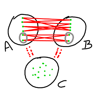
If $H$ is 2-regular then it is almost surely not connected. We can consider the partition induced on $A$ by the components - we call them enclaves. For each enclave in $A$ there is a corresponding enclave in $B,$ and it is easy to see that the 2-colouring on $H$ is not unique, as colours on corresponding enclaves can be swapped.
In the diagram here we see $H$ with two enclaves, two components, and the vertices circled in grey can be given the colour corresponding to the vertices in the other set.
Conjecture: If $H$ is 3-regular then it is almost surely connected.
Given two sets of size $n$, three edge-independent matchings gives a 3-regular bi-partite graph.
Question: Can all 3-regular bi-partite graphs be decomposed into (obviously exactly three) edge-independent matchings?
As an initial exploration of this idea we ran the following experiment.
Generate a random graph $G=G(n,k)$ as follows:
For each graph the program was run 8 times with different initial random seeds. It's plausible that if alternate colouring were present, at least one of those runs would find it.
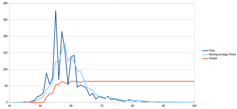
So for each value of $k$ the colouring was run eight times on each of eight different graphs, and if the default colouring was found it was counted. Here is a graph of the results:
|
This clearly shows a correlation between time taken to colour the graph(s) and the onset of probable uniqueness of the colouring. The difficult graphs to colour are the ones with $k$ between 50 and 70, with the peak occurring between 55 and 60. When $k=58$, the average degree is 5.16, which corresponds nicely to the observation of Petford and Welsh.