Please note - this is a pretty quick brain-dump, and some of the questions
and conjectures will, in hindsight, be pretty obvious, or obviously wrong.
We apologise for any inconvenience.
Some preliminaries
We emphasise this occasionally, but for the record:
- All colourings are vertex colourings,
- All graphs are finite,
- A colouring is proper, legal, valid, permitted, and other such words, if
- for every edge $uv$ in $G$, $u$ and $v$ get different colours.
- Usually we are only talking about proper colourings.
- When we say degree we mean the number of edges incident on a vertex.
Where it starts ...
In 1989, A.D.Petford and Dominic Welsh published a paper:
- A Randomised 3-Colouring Algorithm
Their algorithm is roughly:
| This is like a form of simulated annealing (SA).
In SA we pick a random configuration, jiggle it a bit,
if it gets better then keep it (probably), if it gets
worse then don't keep it (probably). As we go on, we
make the probability of accepting a bad change go to
zero.
In the Petford and Welsh algorithm we always accept the
change, but we choose the new colour in such a way as
to make it more likely to be better. The paper suggests
different probability distributions to make that happen,
and examines the effects.
Understanding this is not critical.
|
|
- Randomly colour the given graph
- That is, literally choose a random colour for each vertex
- The colouring need not be "proper" or "legal"
- ... and almost surely will not.
- Repeatedly:
- Choose a vertex at random
- Randomly choose a colour
- based on some probability function $P$ of its neighbours' colours
- Recolour our vertex with this newly chosen colour
- The result will probably still not be proper
- If the graph is now properly coloured:
- If you've been going on for too long:
- Give up, and terminate with failure
We make the following observations:
- Each vertex may be visited many times,
- If we find a colouring then it's valid
- Even if there is a colouring, we might not find it.
In using the algorithm to colour lots of examples they found that with
an appropriate choice of $P$ the algorithm worked quite well.
- This is perhaps unsurprising because most instances of NP-Complete problems are easy to solve.
They did, however, find that there were some graphs that were not
coloured successfully by the algorithm.
Investigating the difficult examples, Petford and Welsh say:
- ... simulations ... tend to confirm our ideas that ...
- for this particular method of colouring ...
- the most difficult case among the class of ...
- roughly regular graphs is the case ...
- when the graphs have low vertex degree, say 5 or 6.
They then go on:
- We have no theoretical explanation of this curious behaviour.
- It is not unlike the phenomenon of phase-transition ...
- which occurs in the Ising model, Potts model ...
- and other models of statistical mechanics.
The concept of "phase transition" is also well known in random graph processes,
perhaps the most common example being the emergence of the giant component.
So the takeaway here is this:
- They have a randomised graph colouring algorithm $\cal A$
- They generate 3-colourable graphs according to a random model
- The random graphs have a parameter
- As they adjust the parameter they look at how long $\cal A$ takes
- The time taken seems linear(ish) but has a strong peak in the mid-range
Idle speculation
Concerning 3-colouring ...
In everything that follows we assume
that the graphs are tri-partite, and
hence guaranteed to be 3-colourable.
|
|
We make some heuristic observations.
Remember:
- We are assuming every graph is tri-partite
- (unless otherwise explicitly stated)
If $G$ has very high average degree then it will almost certainly be easy to
colour. Find any triangle, colour that, then many other vertices will have
their colourings forced, and so the colouring emerges quite quickly.
- For some definition of "quite quickly"
- Remember that by construction we know there is at least one proper 3-colouring.
- We call that colouring the "default" colouring.
This is the case even if there are some vertices of low degree, because the
majority of the graph will have its colouring forced, and the vertices of
low degree will be few in number and not affect the main process.
On the other hand if $G$ has almost no edges then it will almost certainly
be easy to colour, since "most" attempts will work, even if the result is
not the default colouring.
So as the average degree goes from small to large it's plausible to think that
the difficulty of colouring will go from easy, through a peak of difficulty,
and return to being easy.
| The model Petford and Welsh used to generate graphs to test
their colouring algorithm was different. They took $n$ vertices,
coloured them randomly, threw in random edges between differently
coloured vertices, then discarded/forgot the original colouring. |
|
Consider the random graph process where we add the edges of $K_{n,n,n}$ uniformly
at random. We can consider each of the three induced bi-partite graphs and ask
how long it takes for them to become connected. Standard results show that the
onset of connectedness is relatively sharp, but there is an emergence of an
equivalent of the giant component much earlier, so the induced bi-partite
sub-graphs can be thought of as "effectively connected" much earlier.
| In this I'm saying that a graph is "effectively connected" when the
giant component has appeared. In other words, there are a few vertices not
connected to the giant component, but they are few enough in number that we
can ignore them when colouring the graph.
See the page on Effectively Connected.
|
|
The average degree at the onset of full connectedness is much higher than the
observed "5 or 6" quoted in the Petford/Welsh paper, but we might wonder if the
onset of "effective connectedness" is close to that number.
So we observe that in the Erdos-Renyi model of a random 3-colourable graph the
area of difficult instances to colour does not correspond to the emergence
of the connectedness of the induced bi-partite sub-graphs.
Inspiration
Consider the graph $K_{n,n,n}$. Remove all the edges, and then add them back
in one by one in a random order. We can then ask at what point the graph
becomes uniquely 3-colourable. Certainly when any of the induced bi-partite
sub-graphs are not connected the default colouring is not the only one, so
uniqueness of the colouring is much delayed.
But even before the induced bi-partite sub-graphs are connected, they will have
a giant component, and are in a sense "effectively connected". When the giant
component emerges in each of the induced bi-partite graphs, we may regard the
stragglers as hairs that need to be shaved off. This loosely corresponds to
the comment in the Petford/Welsh paper of the graph being "roughly regular."
We can then ask whether the shaved graph is uniquely 3-colourable.
Conjecture: The transition to uniqueness of 3-colouring corresponds closely to
the emergence of the giant components in the induced bi-partite sub-graphs.
Speculation: The peak of difficulty of 3-colouring corresponds closely to the
transition to uniqueness of the colouring.
Analysis
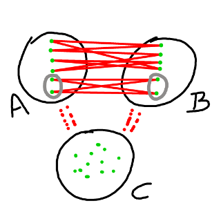
Consider a 3-colourable graph $G$ with colour classes $A$, $B$, and $C$, with
$|A|=|B|=|C|=n$. Consider the induced sub-graph $H\subset G$ on $A{\cup}B.$
We consider whether $G$ is uniquely 3-colourable.
If $H$ is 2-regular then it is almost surely not connected. We can consider the
partition induced on $A$ by the components - we call them enclaves. For each
enclave in $A$ there is a corresponding enclave in $B,$ and it is easy to see
that the 2-colouring on $H$ is not unique, as colours on corresponding enclaves
can be swapped.
In the diagram here we see $H$ with two enclaves, two components, and the vertices
circled in grey can be given the colour corresponding to the vertices in the other
set.
Conjecture: If $H$ is 3-regular then it is almost surely connected.
Given two sets of size $n$, three edge-independent matchings gives a 3-regular
bi-partite graph (and the converse is true ... all 3-regular bi-partite graphs
can be decomposed into (obviously exactly three) edge-independent matchings).
Initial experiment
As an initial exploration of this idea we ran the following experiment.
Generate a random graph $G=G(n,k)$ as follows:
- Take sets $A$, $B$, $C$ with $|A|=|B|=|C|=n$.
- Set $V(G)=A\cup B\cup C$.
- Take a parameter $0\le k\le n$.
- Between each pair:
- Let $m_0$, $m_1$, $m_2$ be edge-independent matchings.
- Put $m_0$ and $m_1$ in $E(G)$.
- Put $k$ edges randomly chosen from $m_2$ in $E(G)$.
Setting $n=100$ and letting $k$ range from 0 to 100, we then generated
8 graphs, and for each of those ran an off-the-shelf graph colouring
program, timing how long it took. The program did not indicate if
the colouring was unique, but a measure was taken of whether the colouring
found was the default colouring present by construction.
For each graph the program was run 8 times with different initial random
seeds. It's plausible that if alternate colouring were present, at least
one of those runs would find it.
So for each value of $k$ the colouring was run eight times on each of eight
different graphs, and if the default colouring was found it was counted.
Here is a graph of the results:
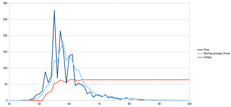
The dark blue line is the average time in seconds taken to colour all of
the 64 graphs. The light blue line is a moving average (and probably not
worth much). The red line is a count of the number of times the default
colouring was found. Its maximum is 64 because for each $k$, that's how
many graphs there are.
This clearly shows a correlation between time taken to colour the graph(s)
and the onset of probable uniqueness of the colouring. The difficult
graphs to colour are the ones with $k$ between 50 and 70, with the peak
occurring between 55 and 60. When $k=58$, the average degree is 5.16,
which corresponds nicely to the observation of Petford and Welsh.
Next experiment ...
The next experiment might be this:
- Take three sets $|A|=|B|=|C|=n$ of vertices.
- For each pair:
- Put two edge-independent matchings
- Take another matching sharing no edges with either of the others.
- Order the edges of the new matching randomly.
- Add the edges one by one in this random order
- At each stage:
- time how long it takes to colour the graph
- Determine if the colouring is unique
- Determine if the induced bi-partite graphs are all connected
Links to this page /
Page history /
Last change to this page
Recent changes /
Edit this page (with sufficient authority)
All pages /
Search /
Change password /
Logout